Thought you were rid of us? Not quite: in a last hurrah, Clément and I come back with a final pair of distribution estimation recaps — this time on results from the actual conference!
Gautam Kamath on Efficient Density Estimation via Piecewise Polynomial Approximation by Siu-On Chan, Ilias Diakonikolas, Rocco A. Servedio, and Xiaorui Sun
Density estimation is the question on everyone’s mind. It’s as simple as it gets – we receive samples from a distribution and want to figure out what the distribution looks like. The problem rears its head in almost every setting you can imagine — fields as diverse as medicine, advertising, and compiler design, to name a few. Given its ubiquity, it’s embarrassing to admit that we didn’t have a provably good algorithm for this problem until just now.
Let’s get more precise. We’ll deal with the total variation distance metric (AKA statistical distance). Given distributions with PDFs  and
and  , their total variation distance is
 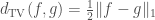 . Less formally but more intuitively, it upper bounds the difference in probabilities for any given event. With this metric in place, we can define what it means to learn a distribution: given sample access to a distribution
  , we would like to output a distribution
  such that
  .
.
This paper presents an algorithm for learning  -piecewise degree-
 polynomials. Wow, that’s a mouthful — what does it mean? A -piecewise degree- polynomial is a function where the domain can be partitioned into intervals, such that the function is a degree- polynomial on each of these intervals. The main result says that a distribution with a PDF described by a -piecewise degree- polynomial can be learned to accuracy
  using
using  samples and polynomial time. Moreover, the sample complexity is optimal up to logarithmic factors.
Now this is great and all, but what good are piecewise polynomials? How many realistic distributions are described by something like “ for
for  but
but  for
for  and
and  …”? The answer turns out to be a ton of distributions — as long as you squint at them hard enough.
The wonderful thing about this result is that it’s semi-agnostic. Many algorithms in the literature are God-fearing subroutines, and will sacrifice their first-born child to make sure they receive samples from the class of distributions they’re promised — otherwise, you can’t make any guarantees about the quality of their output. But our friend here is a bit more skeptical. He deals with a funny class of distributions, and knows true piecewise polynomial distributions are few and far between — if you get one on the streets, who knows if it’s pure? Our friend is resourceful: no matter the quality, he makes it work.
Let’s elaborate, in slightly less blasphemous terms. Suppose you’re given sample access to a distribution  which is at total variation distance
  from some -piecewise degree- polynomial (you don’t need to know which one). Then the algorithm will output a
  -piecewise degree- polynomial which is at distance
  from . In English: even if the algorithm isn’t given a piecewise polynomial, it’ll still produce something that’s (almost) as good as you could hope for.
With this insight under our cap, let’s ask again — where do we see piecewise polynomials? They’re everywhere: this algorithm can handle distributions which are log-concave, bounded monotone, Gaussian, -modal, monotone hazard rate, and Poisson Binomial. And the kicker is that it can handle mixtures of these distributions too. Usually, algorithms fail catastrophically when considering mixtures, but this algorithm keeps chugging and handles them all — and near optimally, most of the time.
The analysis is tricky, but I’ll try to give a taste of some of the techniques. One of the key tools is the Vapnik-Chervonenkis (VC) inequality. Without getting into the details, the punchline is that if we output a piecewise polynomial which is “close” to the empirical distribution (under a weaker metric than total variation distance), it’ll give us our desired learning result. In this setting, “close” means (roughly) that the CDFs don’t stray too far from each (though in a sense that is stronger than the Kolmogorov distance metric).
Let’s start with an easy case – what if the distribution is a  -piecewise polynomial? By the VC inequality, we just have to match the empirical CDF. We can do this by setting up a linear program which outputs a linear combination of the Chebyshev polynomials, constrained to resemble the empirical distribution.
It turns out that this subroutine is the hardest part of the algorithm. In order to deal with multiple pieces, we first discretize the support into small intervals which are roughly equal in probability mass. Next, in order to discover a good partition of these intervals, we run a dynamic program. This program uses the subroutine from the previous paragraph to compute the best polynomial approximation over each contiguous set of the intervals. Then, it stitches the solutions together in the minimum cost way, with the constraint that it uses fewer than  pieces.
In short, this result essentially closes the problem of density estimation for an enormous class of distributions — they turn existential approximations (by piecewise polynomials) into approximation algorithms. But there’s still a lot more work to do — while this result gives us improper learning, we yearn for proper learning algorithms. For example, this algorithm lets us approximate a mixture of Gaussians using a piecewise polynomial, but can we output a mixture of Gaussians as our hypothesis instead? Looking at the sample complexity, the answer is yes, but we don’t know of any computationally efficient way to solve this problem yet. Regardless, there’s many exciting directions to go — I’m looking forward to where the authors will take this line of work!
-G
Clément Canonne on  -Testing, by Piotr Berman, Sofya Raskhodnikova, and Grigory Yaroslavtsev [1])
Almost every — if not all — work in property testing of functions are concerned with the Hamming distance between functions, that is the fraction of inputs on which they disagree. Very natural when we deal for instance with Boolean functions 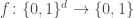 , this distance becomes highly arguable when the codomain is, say, the real line: sure,
 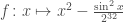 and
and  technically disagree on almost every single input, but should they be considered two completely different functions?
This question, Grigory answered by the negative; and presented (joint work with Piotr Berman and Sofya Raskhodnikova [2]) a new framework for testing real-valued functions ![f\colon X^d\to[0,1]](https://s0.wp.com/latex.php?latex=f%5Ccolon+X%5Ed%5Cto%5B0%2C1%5D&bg=ffffff&fg=404040&s=0&c=20201002) , less sensitive to this sort of annoying “technicalities” (i.e., noise). Instead of the usual Hamming/
, less sensitive to this sort of annoying “technicalities” (i.e., noise). Instead of the usual Hamming/ distance between function, they suggest the more robust (
 ) distance
![\mathrm{d}_p(f,g) = \frac{ \left(\int_{X^d} \lvert f(x)-g(x) \rvert^p dx\right)^{\frac{1}{p}} }{ \left(\int_{X^d} \mathbf{1} dx \right)^{\frac{1}{p}} } = \mathbb{E}_{x\sim\mathcal{U}(X^d)}\left[\lvert f(x)-g(x) \rvert^p\right]^{\frac{1}{p}}\in [0,1]](https://s0.wp.com/latex.php?latex=%5Cmathrm%7Bd%7D_p%28f%2Cg%29+%3D+%5Cfrac%7B+%5Cleft%28%5Cint_%7BX%5Ed%7D+%5Clvert+f%28x%29-g%28x%29+%5Crvert%5Ep+dx%5Cright%29%5E%7B%5Cfrac%7B1%7D%7Bp%7D%7D+%7D%7B+%5Cleft%28%5Cint_%7BX%5Ed%7D+%5Cmathbf%7B1%7D+dx+%5Cright%29%5E%7B%5Cfrac%7B1%7D%7Bp%7D%7D+%7D+%3D+%5Cmathbb%7BE%7D_%7Bx%5Csim%5Cmathcal%7BU%7D%28X%5Ed%29%7D%5Cleft%5B%5Clvert+f%28x%29-g%28x%29+%5Crvert%5Ep%5Cright%5D%5E%7B%5Cfrac%7B1%7D%7Bp%7D%7D%5Cin+%5B0%2C1%5D&bg=ffffff&fg=404040&s=0&c=20201002)
(think of  as being the hypercube
  or the hypergrid
 ![[n]^d](https://s0.wp.com/latex.php?latex=%5Bn%5D%5Ed&bg=ffffff&fg=404040&s=0&c=20201002) , and
, and  being 1 or 2. In this case, the denominator is just a normalizing factor
  or
or  )
)
Now, erm… why?
- because it is much more robust to noise in the data;
- because it is much more robust to outliers;
- because it plays well (as a preprocessing step for model selection) with existing variants of PAC-learning under norms;
- because
 and
and  are pervasive in (machine) learning;
- because they can.
Their results and methods turn out to be very elegant: to outline only a few, they
- give the first example of testing monotonicity testing (de facto, for the distance) when adaptivity provably helps; that is, a testing algorithm that selects its future queries as a function of the answers it previously got can outperform any tester that commits in advance to all its queries. This settles a longstanding question for testing monotonicity with respect to Hamming distance;
- improve several general results for property testing, also applicable to Hamming testing (e.g. Levin’s investment strategy [3]);
- provide general relations between sample complexity of testing (and tolerant testing) for various norms (
 );
);
- have quite nice and beautiful algorithms (e.g., testing via partial learning) for testing monotonicity and Lipschitz property;
- give close-to-tight bounds for the problems they consider;
- have slides in which the phrase “Big Data” and a mention to stock markets appear (!);
- have an incredibly neat reduction between and Hamming testing of monotonicity.
I will hereafter only focus on the last of these bullets, one which really tickled my fancy (gosh, my fancy is so ticklish) — for the other ones, I urge you to read the paper. It is a cool paper. Really.
Here is the last bullet, in a slightly more formal fashion — recall that a function defined on a partially ordered set is monotone if for all comparable inputs  such that
  , one has
  ; and that a one-sided tester is an algorithm which will never reject a “good” function: it can only err on “bad” functions (that is, it may sometimes accept, with small probability, a function far from monotone, but will never reject a monotone function).
Theorem.
Suppose one has a one-sided, non-adaptive tester  for monotonicity of Boolean functions
  with respect to Hamming distance, with query complexity
  . Then the very same is also a tester for monotonicity of real-valued functions
 ![f\colon X\to [0,1]](https://s0.wp.com/latex.php?latex=f%5Ccolon+X%5Cto+%5B0%2C1%5D&bg=ffffff&fg=404040&s=0&c=20201002) with respect to distance.
with respect to distance.
Almost too good to be true: we can recycle testers! How? The idea is to express our real-valued as some “mixture” of Boolean functions, and use as if we were accessing these. More precisely, let ![f\colon [n]^d \to [0,1]](https://s0.wp.com/latex.php?latex=f%5Ccolon+%5Bn%5D%5Ed+%5Cto+%5B0%2C1%5D&bg=ffffff&fg=404040&s=0&c=20201002) be a function which one intends to test for monotonicity. For all thresholds
be a function which one intends to test for monotonicity. For all thresholds ![t\in[0,1]](https://s0.wp.com/latex.php?latex=t%5Cin%5B0%2C1%5D&bg=ffffff&fg=404040&s=0&c=20201002) , the authors define the Boolean function
, the authors define the Boolean function  by
by
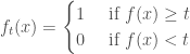
All these are Boolean; and one can verify that for all  ,
,  . Here comes the twist: one can also show that the distance of to monotone satisfies
i.e. the distance of to monotone is the integral of the Hamming distances of the ‘s to monotone. And by a very simple averaging argument, if is far from monotone, then at least one of the ‘s must be…
How does that help? Well, take your favorite Boolean, Hamming one-sided (non-adaptive) tester for monotonicity, : being one-sided, it can only reject a function if it has some “evidence” it is not monotone — indeed, if it sees some violation: i.e., a pair with  but
but  .
.
Feed this tester, instead of the Boolean function it expected, our real-valued ; as one of the  ‘s is far from monotone, our tester would reject ; so it would find a violation of monotonicity by if it were given access to . But being non-adaptive, the tester does exactly the same queries on as it would have done on this ! And it is not difficult to see that a violation for is still a violation for : so the tester finds a proof that is not monotone, and rejects.
Wow.
— Clément.
Final, small remark: one may notice a similarity between testing of functions ![f\colon[n]\to[0,1]](https://s0.wp.com/latex.php?latex=f%5Ccolon%5Bn%5D%5Cto%5B0%2C1%5D&bg=ffffff&fg=404040&s=0&c=20201002) and the “usual” testing (with relation to total variation distance,
and the “usual” testing (with relation to total variation distance,  ) of distributions
 ![D\colon [n]\to[0,1]](https://s0.wp.com/latex.php?latex=D%5Ccolon+%5Bn%5D%5Cto%5B0%2C1%5D&bg=ffffff&fg=404040&s=0&c=20201002) . There is actually a quite important difference, as in the latter the distance is not normalized by
. There is actually a quite important difference, as in the latter the distance is not normalized by  (because distributions have to sum to anyway). In this sense, there is no direct relation between the two, and the work presented here is indeed novel in every respect.
Edit: thanks to Sofya Raskhodnikova for spotting an imprecision in the original review.
[1] Slides available here: http://grigory.github.io/files/talks/BRY-STOC14.pptm
[2] http://dl.acm.org/citation.cfm?id=2591887
[3] See e.g. Appendix A.2 in “On Multiple Input Problems in Property Testing”, Oded Goldreich. 2013. http://eccc-preview.hpi-web.de/report/2013/067/


, which is the best known bound for sparse graphs;
. This algorithm is better for dense graphs.


![f \colon V \to [0, 1]](https://s0.wp.com/latex.php?latex=f+%5Ccolon+V+%5Cto+%5B0%2C+1%5D&bg=ffffff&fg=404040&s=0&c=20201002)


 be a Boolean function of
  (this is tight in the worst case), but a big question in computational complexity is to provide a simple enough function that requires large enough circuits to compute.
 and requires circuits of size super-polynomial in
  , and one of the Millenium Problems is solved!
 ! You may ask: why one should be excited about such a seemingly weak improvement (which, nevertheless, took the authors several years of hard work, as far as I know)?
 space with
  . A cool bonus of this result is that it gives a new technique for obtaining sketching lower bounds.
 that preserves properties of
  -dimensional subspace, and this will preserve with high probability all the pairwise distances up to a factor of
  .
. between two objects
  . Often times similarity between objects is modeled by some
  (but not always! think
  , one is able to estimate the distance
  or
or  (where
  and
and  are the parameters known from the beginning). Both Alice and Bob send messages
  bits long to Charlie, who is supposed to distinguish two cases (whether
  is small or large) with probability at least
  . We assume that all three parties are allowed to use shared randomness. Our main goal is to understand the trade-off between
  we define
  to be a
 this expression should be understood as
  ). One can similarly define
  ; even if the triangle inequality does not hold for this case, it is nevertheless a meaningful notion of distance.
 and sketch size
  for every
  (for
(for  this was
  the dependence on the dimension is necessary. It
  the optimal sketch size is
  .
. is an embedding with distortion
  , if
, if
 and for some
  . It is immediate to see that if a metric space
  , then one can sketch
  and
and  with distortion
  . This result together with the above upper bound by Indyk provides a complete characterization of normed spaces that admit good sketches.
 -threshold, if for every
  implies
  ,
, implies
  .
. -threshold map to a
  (the direct sum of
  ).
). , where
  is a Hilbert space such that
 are non-decreasing functions such that
  for every
  and
and  as
as  . Both
  and
and  are allowed to depend only on
  -squared), but neither of them is embeddable into
  . I do not know, if these spaces are embeddable into
  , where
  is a random matrix generated using shared randomness. Our result then can be interpreted as follows: any normed space that allows sketches of size
  (this follows from the fact that for
  and approximation
  , where
  and
and  are some (ideally, not too quickly growing) functions?
 ? The only example I can think of is a space that contains a subspace that is close to
  . Is this the only case?
 or
or  , but today, and often in the study of Boolean analysis, we will think of functions as mapping
  to
to  , which is roughly equivalent for many purposes (O’Donnell has a nice rule of thumb as when to use one convention or the other
  , we can define two important measures of sensitivity. The first is the average sensitivity (or, for those of you like me who grew up with O’Donnell’s book, the total influence) of the function, namely,
![\mathbb{AS}(f) = \mathbb{E}_{x \sim \{-1, 1\}^n} [| \{i: f(x^{i \to 1}) \neq f(x^{i \to -1}) \} |]](https://s0.wp.com/latex.php?latex=%5Cmathbb%7BAS%7D%28f%29+%3D+%5Cmathbb%7BE%7D_%7Bx+%5Csim+%5C%7B-1%2C+1%5C%7D%5En%7D+%5B%7C+%5C%7Bi%3A+f%28x%5E%7Bi+%5Cto+1%7D%29+%5Cneq+f%28x%5E%7Bi+%5Cto+-1%7D%29+%5C%7D+%7C%5D&bg=ffffff&fg=404040&s=0&c=20201002)
 is simply
  th coordinate set to
  . The second is the noise sensitivity of the function, which is defined similarly: for a parameter
  , it is the probability that if we sample
  . When we generate a string
  -correlated. The weird function of
  .
. , then it turns out that bounds on these two quantities can often be translated directly into learning algorithms for these classes. By Fourier analytic arguments, good bounds on the noise sensitivity of a function immediately imply that the function has good Fourier concentration on low degree terms, which in turn imply that the so-called “low-degree algorithm” can efficiently learn the class of functions in the
  , then the average sensitivity is how many edges cross from one subset into another (over
  ), so it is fundamentally related to the surface area of subsets of the hypercube, which comes up all over the place in Boolean analysis. Secondly, in some cases, we can translate between one measure and the other by considering restrictions of functions. To the best of my knowledge, this appears to be a technique first introduced by Peres in 1999, though his paper is from 2004 [3]. Let
  . We wish to bound the noise sensitivity of
  -correlated to
  for some integer
  , and a
  . Then, for any string
  , we associate it with the string
  whose
whose  times the
  th coordinate of
  . Why are we doing this? Well, after some thought, it’s not too hard to convince yourself that if we choose the
  uniformly at random, then we get a uniformly random string
  , and produce a new string
  and
and  where
where  and for concreteness let’s say
  (however, it’s not too hard to see that any halfspace has a representation so that the linear function inside the sign is never zero on the hypercube). Intuitively, take the hyperplane in
  with normal vector
  , then assign to all points which are in the same side as
  , and the rest
  . Halfspaces are an incredibly rich family of Boolean functions which include arguably some of the important objects in Boolean analysis, such as the dictator functions, the majority function, etc. There is basically a mountain of work on halfspaces, due to their importance in learning theory, and as elementary objects which capture a surprising amount of structure.
 is the function which is
  for all
  as a
as a  predicate on the boolean cube, then their intersection is simply their AND (or NOR, depending on your map from
 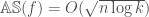 .
. halfspaces with one more can only increase the average sensitivity by a small factor.
 .
. given any input
  such that
  . The existence of one-way functions imply a wide range of fundamental cryptographic primitives, including pseudorandom generation, pseudorandom functions, symmetric-key encryption, bit commitments, and digital signatures – and vice versa: the seminal work of Impagliazzo and Luby [1] showed that the existence of cryptography based on complexity-theoretic hardness assumptions – encompassing the all of the aforementioned primitives – implies that one-way functions exist.
 ) also imply one-way functions. Yet more recently, Haitner and Omri [4] showed that the same holds for any coin-flipping protocol with a constant bias (namely, a bias of
  ). Finally, Berman, Haitner and Tentes proved that coin-flipping of any constant bias implies one-way functions. The remainder of this post will give a flavor of the main ideas behind their proof.
 between players
  and
and  , we first define a (sort of) one-way function, then show that an adversary capable of efficiently inverting that function must be able to achieve a significant bias in
  . The one-way function used is the transcript function which maps the players’ random coinflips to a protocol transcript. The two main neat insights are these:
 be the function that takes as input a pair
  , where
  is a random transcript of a partial (incomplete) honest execution of
  , and outputs a random pair of random coinflips
  for the players, satisfying the following two conditions: (1) they are consistent with
  .
. for each partial transcript
  be the honest first player’s strategy. Now, define
  to be attacker which, rather than sampling a random 1-continuation among all the possible honest continuations of the protocol
  , instead samples a random 1-continuation among all continuations of
  . Note that
  is the biased-continuation attacker described above! It turns out that as the number of recursions grows, the probability that the resulting transcript will land in the “immune” set approaches 1 – meaning a successful attack! Naïvely, this attack may require exponential time due to the many recursions required; however, the paper circumvents this by analyzing the probability that the transcript will land in a set which is “almost immune”, and finding that this probability approaches 1 significantly faster.
 factor in the race for the fastest solver.
 are easier to solve whenever
  , which happens to be a convex function due to the PSD-ness of
  , we care about finding a sparser graph
 (the smaller, the better). The point is that whenever you do gradient descent in order to minimize
  . Of course, this requires another linear system solve, only that this only needs to be done on a sparser graph. Applying this idea recursively eventually yields efficient solvers. A lot of combinatorial work is spent on understanding how to compute these sparser graphs.
 ? We need to find away to efficiently apply the operator
  to
to  for some small real
  . Notice that in order to get
  precision, we only need to take the product of the first
  factors. It would be great if we could approximate matrix inverses the same way. Actually, we can, since for matrices of norm less than
  . At this point we’d be tempted to think that we’re almost done, since we can just write
  , and try to invert
  . However we would still need to compute matrix powers, and those matrices might again not even be sparse, so this approach needs more work.
 to a vector consists of left multiplying by
  . How to do this? One crucial ingredient is the fact that
  is also SDD! Therefore we can recurse, and solve a linear system in
  . You might say that we won’t be able to do it efficiently, since
  level of recursion, the operator we need to apply is
  . A quick calculation shows that if the condition number of
  is
is  , then the condition number of
  is
is  . This means that after
  iterations, the eigenvalues of
  are close to
  , so we can just approximate the operator with
  without paying too much for the error.
 Time
Time be the Laplacian of our given graph, and
  , which converges to the solution of the system. It starts with a weak estimate for the solution, and iteratively attempts to decrease the norm of the residue
  by updating the current solution with a coarse approximation to the solution of the system
  . That coarse approximation is computed using
  . Therefore steps are given by
![\alpha \in (0,1]](https://s0.wp.com/latex.php?latex=%5Calpha+%5Cin+%280%2C1%5D&bg=ffffff&fg=404040&s=0&c=20201002) is a parameter that adjusts the length of the step. The better
is a parameter that adjusts the length of the step. The better  . Unfortunately, in general we don’t know how to achieve this bound yet; the best known result is off by a
  factor. It turns out that we can still get preconditioners by looking at a different quantity, called the
  . This essentially eliminates the need for computing optimal low stretch spanning trees. Furthermore, these trees can be computed really fast,
  time in the RAM model, and the algorithm parallelizes.
 is also known as the Lowner partial order.
  is equivalent to
  , which says that
  is PSD.
 -ultrasparsifier
  edges such that
  . It turns out that one is able to efficiently construct
  ultrasparsifiers. So by adding a few edges to a spanning tree, you can drastically reduce the relative condition number with the initial graph.
 -Time Spectral Algorithm for Balanced Separator
